PET and MRI as devices of CBF measurement
Computer-based tomographic techniques originated with the invention of x-ray computed tomography (CT) scanner by Hounsfield in 1972 [1]. Those techniques were applied to the field of nuclear medicine, and paved the way for the development of new imaging modalities, including positron emission tomography (PET and nuclear magnetic resonance imaging (NMRI), that utilize the phenomenon of nuclear magnetic resonance. In the subsections to follow, we will discuss how these two imaging methods were developed, and what their imaging characteristics are. The major differences between the PET and MRI images of cerebral blood flow will also be discussed.
1. Basic Principles of Tomography
1-1. Principles of CT
Since Roentgen’s discovery of x-rays in 1895, the primary thrust of x-ray diagnostics has been to project and record a shadow of an object onto radiation-sensitive film. These techniques are intended to obtain internal information about the object, based on the differences in x-ray absorption profile among the materials along the beam trajectory. However, these methods are not suitable for in-depth investigation of the internal structure, because the shadows of all internal components are projected onto a single plane, resulting in a significant loss of valuable information.
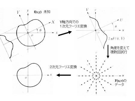
The reconstitution methods for CT data have been constantly evolving since the CT technique was invented. Initially, these methods were developed for analysis of x-ray projection data.The Fourier transform is the core of algorithms for tomographic reconstitution (i.e., three-dimensional reconstitution), which have been applied to both PET and MRI imaging analysis. Real and Fourier spaces are interconvertible via the Fourier transform; thus, sampling of Fourier space can lead to the reconstitution of real space. In the case of x-ray CT measurements, projection data obtained in real space is converted to Fourier components for the purposes of data processing.
The two-dimensional Fourier transform of a continuous function  can be defined as <*1>:
When v = 0, we have:
where  designates a projection of along the y-axis onto the x-axis. This means that taking the one-dimensional Fourier transform of projection data along the y-axis yields a line of data in Fourier space that passes along the same direction as the projection line, crossing the origin.
This holds true for projections in any direction [2].
We can obtain lines in Fourier space for any angle by calculating one-dimensional Fourier transforms in a similar manner. The real-space data can be derived by applying the inverse two-dimensional Fourier transform to the resulting Fourier-space data (Fig. 1).
In the case of an x-ray CT measurement, designates the x-ray absorption coefficient at (x,y); this function represents the absorption of x-rays along the beam path, and can be expressed as:
Absorption = Log [(x-ray source intensity)/(x-ray detector intensity)].
The filtered back-projection method, which is a mathematically equivalent process to that described above, is commonly used in actual CT scan settings.
<*1> Using a vector representation, this equation can be expressed as:  where the symbol “・”designates the inner product.
|
Fig. 1 Principles of x-ray CT image reconstruction.
f(x,y) unknown One-dimensional Fourier transform along the Y-axis
Repeat multiple times by changing the angle of projection.
F(u,v) data Two-dimensional Fourier transform
 |
1-2. PET
PET (positron emission tomography) detects gamma rays emitted by the collision of a positron and an electron, in order to determine the spatial distribution of the PET tracer. Knowledge of the overall spatial distribution of the tracer allows the construction of two- and three-dimensional medical images. Selection of appropriate tracers enables various physical and biochemical measurements (e.g., glucose metabolism, cerebral blood flow, blood volume, oxygen metabolism, neural receptor distribution). As in CT, the filtered back-projection method is commonly used for PET image reconstruction, in which case function designates the positron probability density. The projection data are obtained by preprocessing raw gamma-ray data, including (1) attenuation correction, (2) correction for scattered and random coincidences, and (3) count-rate linearity correction. Projection data are further subjected to cross-calibration in order to quantitatively determine the local distribution of the positron-emitting radiological markers, used in tomographic image reconstruction (refer to references [3] to [5] for more details)
(1) Attenuation Correction
Coincidence measurements allow for accurate attenuation correction, regardless of the location of the positron-emitting source within the object. When a positron-electron collision occurs at depth d within the object, a pair of annihilation gamma rays are emitted in opposite directions; their energies are absorbed along the travel path t. The probability for the both rays to be detected is equal to the product of the individual probabilities of each gamma ray reaching the PET detector.When we assume that μ(t) is the attenuation coefficient for 511 keV gamma rays along travel path t, we have:
where L is the total length of the path t within the object. This equation indicates that attenuation of the gamma rays depends solely on L, the length of path t, and μ(t), irrespective of the location of the collision site.It follows that attenuation correction relies solely on information about the distribution of the attenuation coefficient μ(x,y) along the line of response; this can be obtained separately by transmission scanning.
(2) Random and Scattered Coincidences
A random coincidence refers to a situation in which two gamma rays originating from different decay events are detected within the coincidence time window, and a scattered coincidence occurs when at least one of the detected photons has undergone a Compton scatter interaction in tissue prior to detection. Two basic approaches are available for the correction of random coincidences: use of a delayed circuit, and estimation of the random coincidence count rate using the single detector rates of the two detectors. Scattered coincidence counts cannot be corrected analytically using theoretical algorithms; instead, in most cases they are empirically compensated for by subtracting the auxiliary data estimated from the scattered counts measured in the vicinity of the object, under the assumption that they represent true scattered counts.
(3) Correction for Count Loss (Count Rate Performance)
Count loss arises from system dead time. The methods for count loss correction vary by system, because the details depend on the type of detector and the design of the circuits that process output signals from the detectors.
(4) Cross-calibration for Absolute Measurement Sensitivity
Physical phantoms with a known dose distrib
|
Fig. 2 Coincidence measurement of PET annihilation gamma rays
Detector 1
ution are used to cross-calibrate the PET scanner and convert the voxel values into corresponding doses.
 |
1-3 MRI
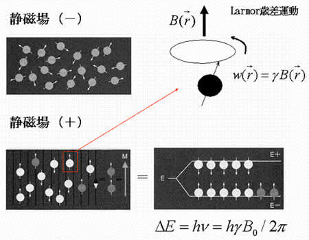
MRI (magnetic resonance imaging) spectroscopy utilizes the nuclear magnetic resonance of protons in order to produce medical images. Each proton possesses an intrinsic spin, which produces a magnetic field. In the absence of an external magnetic field, the direction of the spin is randomly distributed. When a strong external static magnetic field is applied, however, the protons align either with or against the field, resulting in two different energy levels (states). The protons are continually oscillating back and forth between the two states. On a large scale, however, there will always be a slight majority of spins aligned parallel to the field. Consequently, magnetization vectors (spin isochromats) that correspond to local magnetic fields <*2> are formed. The spin rotates around the axis of the external static magnetic field (Larmor precession). The precession angular velocity ( , Larmor frequency) at the instantaneous position of the particle (represented as
  in three-dimensional coordinate system) is proportional to the static magnetic field :
where the proportionality constant  designates the gyromagnetic ratio intrinsic to hydrogen atom (42.6 MHz/T).
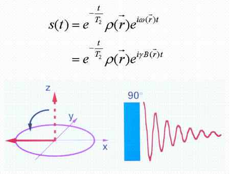
Spins, when subjected to a pulse (electromagnetic wave <*3>) at their Larmor frequency, will absorb the energy and generate transverse magnetization, rotating away from the axis of the main magnetic field (excitation). When the excitation pulse is turned off, the magnetization vectors will return to the axis of the main static field (relaxation). The process of absorption and re-emission of electromagnetic energy is termed ‘nuclear magnetic resonance.’ The behavior of the relaxation process can be detected with a receiver coil placed parallel to the main field, which measures the transverse component of the rotation as a gradually decreasing alternating current. The temporal profile of the attenuation is termed the ‘free induction decay’ (FID) of the MR signal (Fig. 4).If we express the proton density at a position as  , the FID signal function
  can be defined as follows:
where T2 represents the transverse relaxation time (see below).
<*2> The local field must satisfy the following conditions:
Spins in the local area are subject to a uniform magnetic field (i.e., precessing at the same frequency).
The number of the spins in the local area is large enough to allow for the application of statistical mechanics to deal with the behavior of the spin population.
<*3> The excitation pulse is sometimes called a radio frequency (RF) pulse or radio wave, because its frequency is in the range of FM waves.
|
Fig. 3
No static magnetic field (-)
Static magnetic field applied (+)
Larmor precession
 |
|
Fig. 4. Free induction decay.
In NMR the behavior of the transverse component of the magnetization vector can be detected as a gradually attenuating alternating current in a local field that satisfies the following conditions:
|
When the duration of the measurement is short enough relative to T2, the term describing the signal decay,  , can be handled as a constant. Therefore, in the discussion to follow, we re-express the above equation as:
The observed signal S(t), which is the sum of all MRI signals emitted from a tissue (volume:V), can be expressed as:
MR signals released from an object in a uniform magnetic field provide no information about their locations. In order to create a tomographic representation of the object, it is necessary to obtain data regarding the location from which the MR signals are emitted. For this purpose, we introduce a linear gradient magnetic field.
As shown by the equations above, the topology of the object can be determined from differences arising in the magnetic field when a linear gradient is applied to a static magnetic field. The precession angular velocity is proportional to the magnitude of the magnetic field:
Therefore, the position of the magnetic moment can be identified based on the differences in the angular velocity (Fig. 5). This permits the FID signal to represent topological information as a difference in angular velocity:
Now let us define  . This term is the product of the magnetic gradient at the time of measurement and the gyromagnetic ratio, expressed in units of reciprocal distance. Then we have:
During the demodulation process, the carrier wave  will be removed, leaving only the MR signals <*4>:
This formula indicates that the FID function is a Fourier transform of the proton density distribution  . Since this equation is a function of
  , the Fourier space data resulting from the Fourier transform of the proton density distribution is sometimes termed ‘k-space’ data. Thus, k-space data acquired from measurements of FID, made by applying the appropriate linear gradients, is subjected to reverse Fourier transform in order to produce a topographic presentation of proton densities. There are a wide variety of data acquisition methods available for the purpose of filling k-space. Thus, human MRI images created in this manner represent the distribution of hydrogen atoms, indicating differences in tissue composition and the relaxation time of atoms in the tissue (Fig. 6).
<*4> MR signals are sometimes called audio waves because their frequencies are in the hearing range.
|
Fig. 5
By applying a linear gradient magnetic field, topological information can be embedded in pulse frequency data.
 |
|
Fig. 6
FID signal function at location r:
(units:reciprocal distance)
The measured FID signal is the sum of all signals transmitted:
Carrier radiofrequency wave to be eliminated during detection process.
 |
Relaxation Time
As explained above, relaxation is the process by which a magnetization vector (spin isochromat) returns to the direction of the main magnetic field after being energized by an excitation magnetic field. There are two types of relaxation processes—longitudinal and transversal.
The spins rotate around the axis of the external statistic magnetic field (Larmor precession). The magnetization vector is characterized by the thermodynamic equilibrium between the thermal environment (heat bath or lattice) and the spin. In the absence of excitation, only the longitudinal component of the magnetization is detectable, due to the lack of a transverse component resulting from spin-phase coherence. When radiofrequency (RF) excitation (electromagnetic pulse) is applied, some of the spins absorb the energy and shift to a higher energy state (Zeeman level), aligning against the main field, i.e., they form a longitudinal vector component anti-parallel to the main static field. RF waves with a uniform phase (phase coherence) are used for excitation. When the sample is excited with phase-coherent RF pulses, the spins achieve phase coherence when shifting from lower to higher Zeeman levels, and the phase coherence lends itself to the generation of the transverse component of magnetization. The process of relaxation is just the opposite. ‘Longitudinal relaxation’ is the process whereby the spins release their excitation energy to the lattice, and is observed as a recovery of longitudinal magnetization (time constant: T1). On the other hand, ‘transverse relaxation’ refers to the process whereby the spins lose phase coherence; it is observed as the dissipation of the transverse component of magnetization (time constant, T2; Fig. 7). (For more on the quantum mechanical theory of resonance and relaxation, see reference [6].)The values of T1 and T2 depend on the type of tissue under study. Choice of appropriate T1 and T2 values will help create T1- and T2-weighted images, which are useful for differentiating the tissue and the determination of other properties (Fig. 8). These features mark a distinct contrast to the PET images derived based on the pharmacokinetics of radioactive agents.
|
Fig. 7. Spin relaxationFID
Transverse magnetization is achieved via spin-phase coherence of the spins constituting spin isochromats. ‘Transverse relaxation’ refers to the process of losing coherence.
Longitudinal magnetization results from thermodynamic equilibrium between the thermal environment (heat bath, lattice) and the spin. ‘Longitudinal relaxation’ refers to the process of a spin emitting its activation energy into the lattice.
Spin
Time
 |
|
Fig. 8
TE, T2 relaxation, and T2 contrast
Substance with long T2 (e.g., water)
Substance with short T2 (e.g., brain, liver)
Long echo times (TE) maximize T2 contrast.
TR, T1 relaxation, and T1 contrast
Substance with short T1 (e.g., fat)
Substance with longT1 (e.g., water)
Short repetition times (TR) maximize T1 contrast.
 |
2. Brain Activity and Cerebral Blood Flow
Brain activation studies often focus on changes in cerebral blood flow, based on the premise that energy consumption resulting from neural activity is related to local changes in cerebral blood flow. In such studies the pattern of cerebral blood flow is compared between task performance and a matched control condition (often, a resting state in which the subject is not engaged in the task of interest), in order to locate task-induced blood flow changes in a specific brain region. By assuming that the regions exhibiting significant changes in blood flow are associated with the performance of the task, the site of neural activities involved in the task can be identified.
2-1. Cerebral Blood Flow Measurement by PET
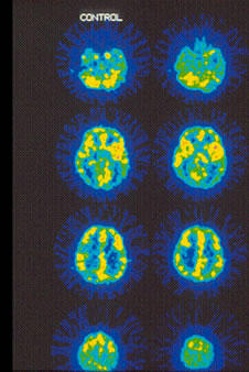
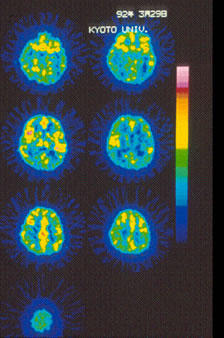
Measurements of human cerebral blood flow using 133Xe gas started in the 1960s [8]. In the 1980s, the PET method for quantitatively determining local changes in cerebral blood flow was established (Fig. 9) [9]. In this method, PET measurements are conducted for 90-120 seconds after a single intravenous injection of 15O-labeled water (half-life: 2 minutes). Simultaneously, arterial blood samples are collected in order to determine the change in blood radioactivity over time. A differential equation is formulated based on a one-compartment model, and used to create a lookup table for the purpose of converting the measured radioactivity to cerebral blood flow, in order to create brain slice images depicting the absolute local cerebral blood flow (Fig. 10). In studies of higher brain function, 15O-labeled water has been widely employed because it helps to repeat measurements within a short period of time.
|
Fig. 9
Basic principles of PET determination of cerebral blood flow using 15O-labeled water and a one-compartment model.
Input data for local cerebral radioactivity concentration CT(t) are taken from PET measurements, while data for the input function Ca(t) are obtained from arterial blood sampling.
|
|
Fig. 10.
15O-water PET images showing cerebral blood flow changes.
|
2-2. Functional MRI (fMRI)
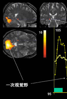
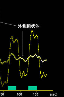
Along with the development of fast MRI techniques, the 1990s brought the development of fMRI approaches that took advantage of endogenous oxygen as a contrast agent. fMRI imaging is sometimes referred to as a blood oxygen level-dependent (BOLD) method, because this technique detects subtle, local signal changes resulting from intravascular oxygenation/deoxygenation that occur in association with neural activation. Oxygenated and deoxygenated hemoglobin have long been known to exhibit different magnetic properties.[10] The presence of deoxygenated hemoglobin in a vessel causes magnetic inhomogeneity in its vicinity. The local magnetic inhomogeneity suppresses the NMR signals relative to the case of magnetic homogeneity. During neural activation the local proportion of deoxygenated hemoglobin decreases, as increased blood flow provides an oxygen supply that surpasses the tissue oxygen demand, thereby enhancing the MNR signals.[11] The advantages of this method include the absence of radiation exposure and the short periods of measurement time required to record the blood flow data for the entire brain. In addition, fMRI can collect a far larger amount of data than PET (Fig. 11). On the other hand, the method also has disadvantages: only changes in blood flow are detectable, and no absolute measurements can be provided.
|
Fig. 11
Illustration of fMRI scans obtained using a 3-tesla MRI system.
The images show brain activation (i.e., lateral geniculate body and primary visual cortex) in an individual presented with an 8-Hz flashing light stimulus.
Lateral geniculate body
Primary visual cortex
  |
Past fMRI studies of brain activation in healthy adult volunteers have shown that the observed signal enhancement correlated well with the local increase in cerebral blood flow and neural activity. In addition, direct comparison of fMRI and PET scans from the same subjects has revealed a high correlation of activity levels in the brain.
It is important to bear in mind that these techniques can detect magnitudes of change that represent ‘gaps’ between the level of oxygen supplied by cerebral blood flow and the level of oxygen consumed by neural activities (Fig. 12). For example, in the early period of life, the human brain undergoes rapid morphological, functional, and metabolic development. The number of synapses of the visual cortex, in particular, starts to grow exponentially two months after birth, culminates in a peak in eight to nine months, and thereafter gradually decreases to the adult level, which is similar to the number at birth.[12] Researchers have found that stimulus-related changes in MR signals in the primary visual cortex is positive in infants younger than two months, but negative in those older than two months.[13, 14] The change observed in older infants was opposite to the change generally observed in adults. The original authors have concluded that the observed inversion is related to the increased demand for oxygen owing to rapid synaptogenesis.
At present, a large amount of research has been performed on brain activation in adults using cerebral blood flow as an indicator of regional brain activity. Ongoing work in this field forms the mainstream of systems neuroscience. A summary comparison of PET and fMRI methodologies is presented in Fig. 13.
|
Fig. 12
 |
|
Fig. 13
 |
References
- Hounsfield GN. Computerized transverse axial scanning (tomography). 1. Description of system. Br J Radiol 1973; 46: 1016-22.
- 英保茂 システム制御情報ライブラリー5 医用画像処理 朝倉書店 1997
- 田中栄一 三次元アイソトープ像の計測と画像再構成 Radioisotopes 39:510-520, 1990
- 村山秀雄 陽電子の科学と計測シリーズ VIII ポジトロン・エミッション・トモグラフィ 3.画像の再構成とデータ補正 Radioisotopes 42+ 244-254 1993.
- 鳥塚莞爾監修 クリニカルPET 先端医療技術研究所 1997
- 荒田洋治 NMRの書 丸善 2000
- Raichle ME. Circulatory and metabolic correlates of brain function in normal humans. Handbook of Physiology. Vol Section 1: The Nervous System. Volume V. Higher Functions of the Brain. Bethesda: Am. Physiol. Soc., 1987: 643-674.
- Lassen NA, Ingvar DH. Radioisotope assessment of regional cerebral blood flow. Prog Nucl Med 1972; 1: 376-409.
- Herscovitch P, Markham J and Raichle M. Brain blood flow measured with intravenous H215O I. Theory and error analysis. J Nucl Med 24: 782-789, 1983.
- Pauling L, Coryell C. The magnetic properties of and structure of hemoglobin, oxyhemoglobin and carbonmonoxyhemoglobin. Proc Natl Acad Sci U S A 1936;22:210-216.
- Ogawa S, Lee TM, Kay AR, Tank DW. Brain magnetic resonance imaging with contrast dependent on blood oxygenation. Proc Natl Acad Sci U S A 1990;87 (24):9868-72.
- Huttenlocher P, deCourten C, Gray L, Loos Hvd. Synaptogenesis in human visual cortex- evidence for synapse elimination during normal development. Neurosci Lett 1982;33:247-252.
- Yamada H, Sadato N, Konishi Y, Muramoto S, Kimura K, Tanaka M, et al. A milestone for normal development of the infantile brain detected by functional MRI. Neurology 2000; 55: 218-23.
- Morita T, Kochiyama T, Yamada H, Konishi Y, Yonekura Y, Matsumura M, et al. Difference in the metabolic response to photic stimulation of the lateral geniculate nucleus and the primary visual cortex of infants: a fMRI study. Neurosci Res 2000; 38: 63-70.